In this post, I will try to give an intuition on how backpropagation works and what factors affect this process. First of all, backpropagation is the process of applying the chain rule from calculus. You can learn more about the chain rule here.
Why do we need backpropagation?
We use backpropagation to compute the gradient of the cost function \(J\) with respect to learnable parameters like \(W\) and \(b\)
\[\frac{dJ}{dW} , \frac{dJ}{db}\]these gradients give us insight on how the cost function will response if we slightly increased the value for the learnable parameters by a small value epsilon.
so if \(\frac{dJ}{dw}\) is +2 then if we increased w in a small value epsilon \(\epsilon\) the cost function J will increase by \(2 \times \epsilon\).
\[J(w + \epsilon) = J(w) + 2 \times \epsilon\]so the derivative is equal to k in this formula:
\[f(x + \epsilon) = f(x) + k \times \epsilon\]since the gradients tell us how the cost function will respond when there value increases, we want to adjust there values in the opposite side, because we want to minimize J. If the gradient is positive let’s say +2 for example then we need to make the value of the parameter smaller. But if the gradient is negative like -2 that means increasing this gradient by epsilon will make J decrease by \(2 \times \epsilon\) and that’s what we want (decrease the cost).
and the sentence above can be translated as:
\[w := w - \frac{dJ}{dw}\] \[b := b - \frac{dJ}{db}\]then we do the same thing over and over, calculate the new cost then calculate the gradients and update the parameters.
as we repeat that process the parameters will get updated and cost will decrease and that’s eventually what we call “training a model”.
To make learning more stable, we introduce a learning rate \(\alpha\) leading to the well-known gradient descent algorithm:
\[w := w - \alpha \times \frac{dJ}{dw}\] \[b := b - \alpha \times \frac{dJ}{db}\]So, backpropagation is a way to compute the gradients of cost function with respect to the learnable parameters to update the learnable parameters in a way that would decrease the cost function.
Let’s now see how this process will occur in a neural network.
consider this simple neural net:
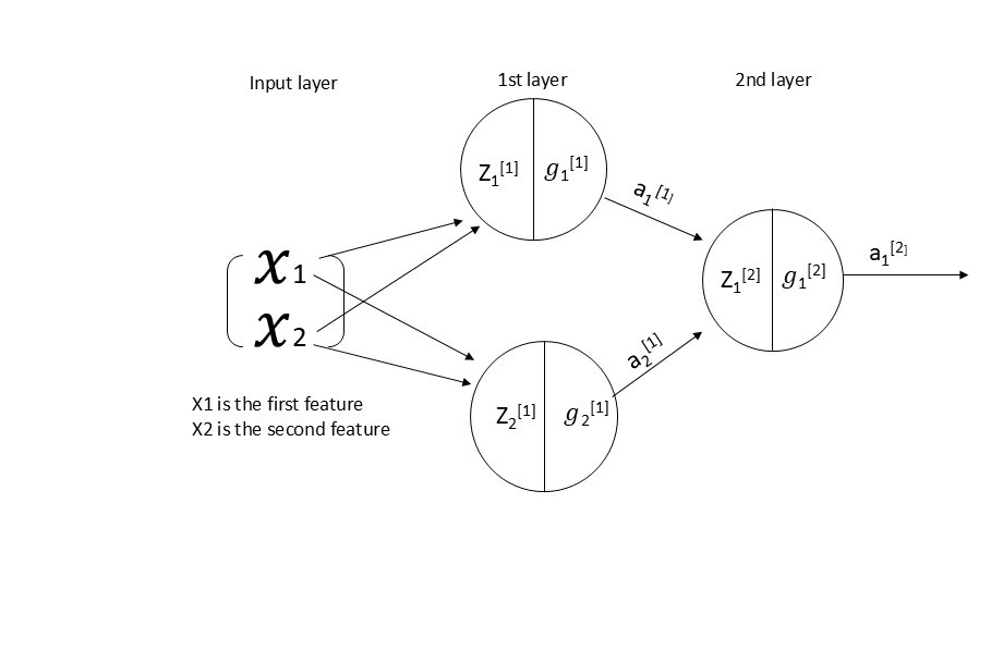
Image by the author.
Neural Networks are functions (a very complex one). They have input x this input goes through the function and apply mathematical operation on it then we get the output \(\hat{y}\). This procedure of inputting x and getting \(\hat{y}\) we call it forward pass in the neural network.
then we compute the cost function by comparing \(y\) to \(\hat{y}\) on \(m\) example.
After getting the cost function, now we can calculate the gradients using backpropagation and this is the backward pass.
how can we apply backpropagation in a neural network?
we are going to start from the cost function, compute the gradients with respect to the expressions that led us to the cost one by one until we reach the learnable parameters(chain rule).
if you didn’t understand what i said it’s ok every thing will be more clear after the example.
I said that we need to compute the gradient of cost with respect to the expressions(mathematical expressions) that led us to the cost.We represent these mathematical expressions by something called Computational Graph.
Computational graphs are directed graphs where the nodes correspond to mathematical operations.
A computational graph is not exclusive to neural networks., any function can be written as a Computational Graph.
For example:
if we want to represent \(y = 2\times x+4\) the computational graph would be like this :
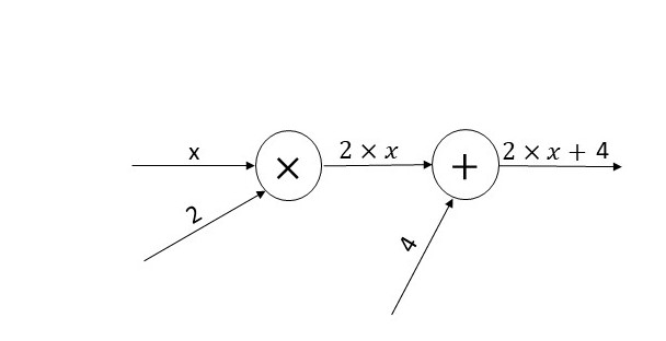
Image by the author.
Given this equation
\[y = 2 \times x + 4\]we know from calculus rules that the derivative of this is :
\[\frac{dy}{dx} = 2\]we can reach the same result by backpropagating through the computational graph:
\[\frac{d(2 \times x + 4)}{d(2 \times x + 4)} = 1\] \[\frac{d(2 \times x + 4)}{d(2 \times x)} = \frac{d(2 \times x + 4)}{d(2 \times x + 4)} \times \frac{d(2 \times x + 4)}{d(2 \times x)}\] \[= 1 \times 1 = 1\] \[\frac{d(2 \times x + 4)}{d(x)} = \frac{d(2 \times x + 4)}{d(2 \times x)} \times \frac{d(2 \times x)}{dx}\] \[= 1 \times 2 = 2\]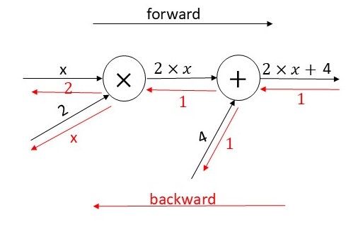
Image by the author.
let’s take more complex example:
\[z = (3 \times x + 4 \times y)^3\]the computational graph is :

Image by the author.
To calculate \(\frac{dz}{dx}\) from calculus rules the result is :
\[\frac{dz}{dx} = 3 \times 3 \times (3 \times x + 4 \times y) ^ 2\] \[= 9 \times (3 \times x + 4 \times y) ^ 2\]Using backpropagation we should get same results let’s see:
\[\frac{dz}{dz} = 1\] \[\frac{dz}{d(4 \times y + 3 \times x)} = \frac{dz}{dz} \times \frac{dz}{d(4 \times y + 3 \times x)}\] \[= 1 \times (3 \times \ (4 \times y + 3 \times x)^2)\] \[= 3 \times \ (4 \times y + 3 \times x)^2\] \[\frac{dz}{d(3 \times x)} = \frac{dz}{d(4 \times y + 3 \times x)} \times \frac{d(4 \times y + 3 \times x)}{d(3 \times x)}\] \[= 3 \times \ (4 \times y + 3 \times x)^2 \times 1\] \[= 3 \times \ (4 \times y + 3 \times x)^2\] \[\frac{dz}{dx} = \frac{dz}{d(3 \times x)} \times \frac{d(3 \times x)}{d(x)}\] \[= 3 \times \ (4 \times y + 3 \times x)^2 \times 3\] \[= 9 \times \ (4 \times y + 3 \times x)^2\]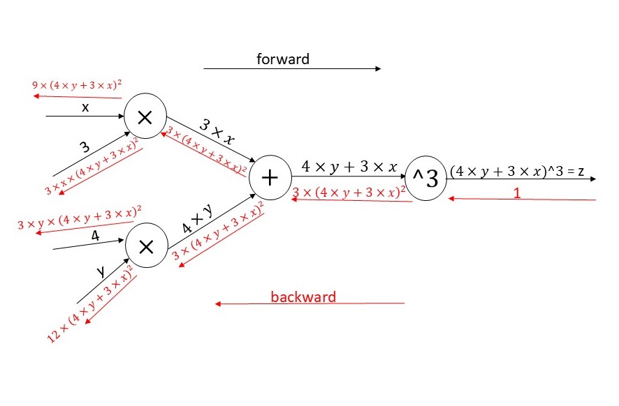
Image by the author.
now let’s represent the neural network as computational graph, and for simplicity consider \(g\) is a linear activation (no activation) in the first and second layer :

Image by the author.
now let’s illustrate the backward pass:
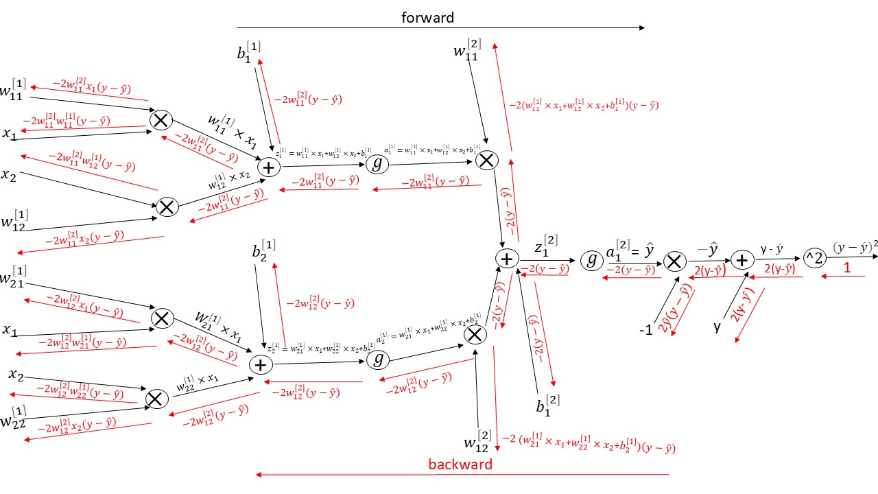
Image by the author.
you can see how complex it is for a neural network with two layers of three units.You can imagine how big it is for deep neural network with hundreds of layers and thousand of units(neurons).
so we build these computation graphs to get the derivative of any function using the chain rule.
if we look at the derivative of the loss with respect to \(x_{2}\) equals :
\[-2w_{12}^{[2]}w_{22}^{[1]}(y - \hat{y})\]The derivative multiply to weights from different layers with each other.If the neural network consist of ten layers or more the derivatives that flow backward know multiply ten weights with each others or more.This will lead us to the problem of vanishing and exploding gradients.
if the weight were big numbers the gradient will become very big in more shallow layers(first layers) because as I said before we will multiply different weights with each others. In the other side, if the weights are close to zero then the gradient will vanish (becomes zero).
Last note: To be more precise the gradient of the loss with respect to \(x_{2}\) is the sum of all the gradients flowing back to that node.As shown in the diagram, two gradients flow back to \(x_{2}\), so we sum them:
\[-2w_{12}^{[2]}w_{22}^{[1]}(y - \hat{y}) + (-2w_{11}^{[2]}w_{12}^{[1]}(y - \hat{y}))\]